pacman::p_load(igraph, tidygraph, ggraph, visNetwork, lubridate, clock, tidyverse, graphlayouts,readr,dplyr,ggplot2)Hands-on Exercise 9: Visualising and Analysing Text Data
1 Getting Started
1.1 Install and loading R packages.
2 Importing Data
GAStech_nodes <- read_csv("../../data/GAStech_email_node.csv")
GAStech_edges <- read_csv("../../data/GAStech_email_edge-v2.csv")
2.1 Wrangling time
Click to view the code.
GAStech_edges <- GAStech_edges %>%
  mutate(SendDate = dmy(SentDate)) %>%
  mutate(Weekday = wday(SentDate,
                        label = TRUE,
                        abbr = FALSE))
2.2 Wrangling attributes
3 Creating network objects using tidygraph
3.1 Using tbl_graph() to build tidygraph data model
Click to view the code.
GAStech_graph <- tbl_graph(nodes = GAStech_nodes,
                           edges = GAStech_edges_aggregated,
                           directed = TRUE)
3.2 Reviewing the output tidygraph’s graph object
GAStech_graph# A tbl_graph: 54 nodes and 1372 edges
#
# A directed multigraph with 1 component
#
# Node Data: 54 × 4 (active)
id label Department Title
<dbl> <chr> <chr> <chr>
1 1 Mat.Bramar Administration Assistant to CEO
2 2 Anda.Ribera Administration Assistant to CFO
3 3 Rachel.Pantanal Administration Assistant to CIO
4 4 Linda.Lagos Administration Assistant to COO
5 5 Ruscella.Mies.Haber Administration Assistant to Engineering Group Mana…
6 6 Carla.Forluniau Administration Assistant to IT Group Manager
7 7 Cornelia.Lais Administration Assistant to Security Group Manager
8 44 Kanon.Herrero Security Badging Office
9 45 Varja.Lagos Security Badging Office
10 46 Stenig.Fusil Security Building Control
# ℹ 44 more rows
#
# Edge Data: 1,372 × 4
from to Weekday Weight
<int> <int> <ord> <int>
1 1 2 星期日 5
2 1 2 星期一 2
3 1 2 星期二 3
# ℹ 1,369 more rows3.3 Changing the active object
Click to view the code.
GAStech_graph %>%
  activate(edges) %>%
  arrange(desc(Weight))
# A tbl_graph: 54 nodes and 1372 edges
#
# A directed multigraph with 1 component
#
# Edge Data: 1,372 × 4 (active)
from to Weekday Weight
<int> <int> <ord> <int>
1 40 41 星期六 13
2 41 43 星期一 11
3 35 31 星期二 10
4 40 41 星期一 10
5 40 43 星期一 10
6 36 32 星期日 9
7 40 43 星期六 9
8 41 40 星期一 9
9 19 15 星期三 8
10 35 38 星期二 8
# ℹ 1,362 more rows
#
# Node Data: 54 × 4
id label Department Title
<dbl> <chr> <chr> <chr>
1 1 Mat.Bramar Administration Assistant to CEO
2 2 Anda.Ribera Administration Assistant to CFO
3 3 Rachel.Pantanal Administration Assistant to CIO
# ℹ 51 more rows4 Plotting Practice - Plotting Static Network Graphs with ggraph package
4.1 Plotting a basic network graph
Click to view the code.
ggraph(GAStech_graph) +
  geom_edge_link() +
  geom_node_point()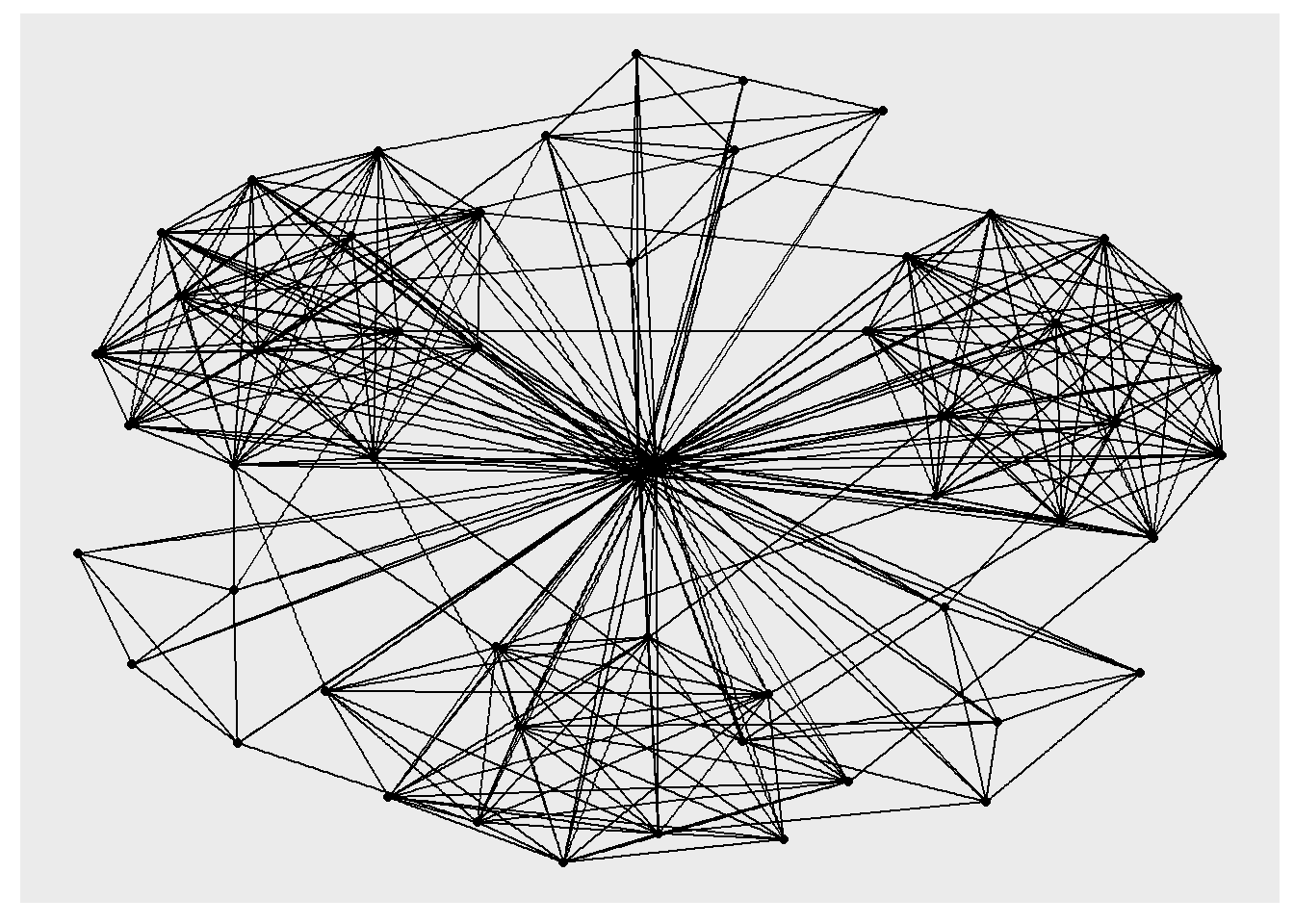
4.2 Changing the default network graph theme
Click to view the code.
g <- ggraph(GAStech_graph) +
  geom_edge_link(aes()) +
  geom_node_point(aes())

g + theme_graph()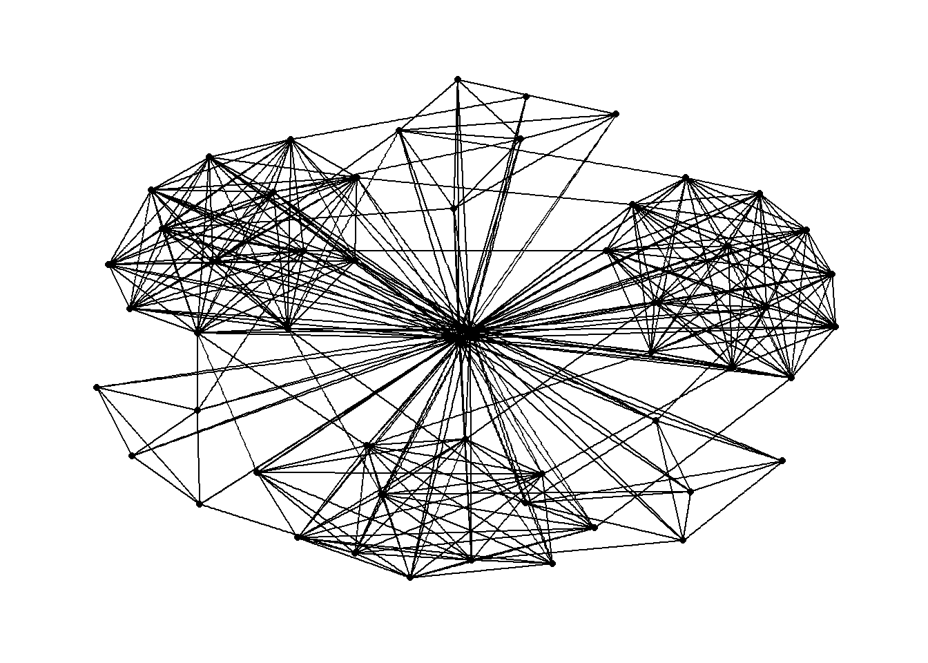
4.3 Changing the coloring of the plot
Click to view the code.
g <- ggraph(GAStech_graph) +
  geom_edge_link(aes(colour = 'grey50')) +
  geom_node_point(aes(colour = 'grey40'))

g + theme_graph(background = 'grey10',
                text_colour = 'white')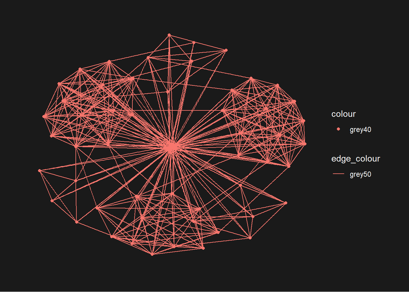
4.4 Fruchterman and Reingold layout
Click to view the code.
g <- ggraph(GAStech_graph,
            layout = "fr") +
  geom_edge_link(aes()) +
  geom_node_point(aes())

g + theme_graph()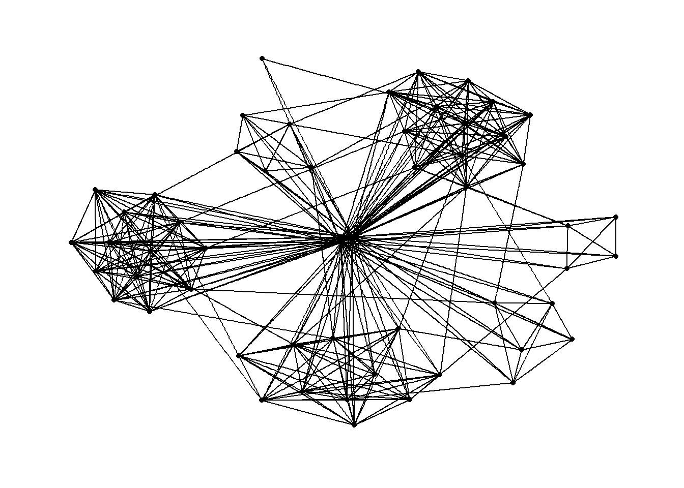
4.5 Modifying network nodes
Click to view the code.
g <- ggraph(GAStech_graph,
            layout = "nicely") +
  geom_edge_link(aes()) +
  geom_node_point(aes(colour = Department,
                      size = 3))

g + theme_graph()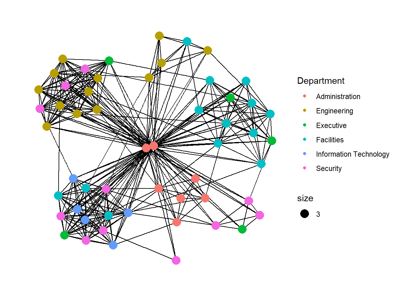
4.6 Modifying edges
Click to view the code.
g <- ggraph(GAStech_graph,
            layout = "nicely") +
  geom_edge_link(aes(width=Weight),
                 alpha=0.2) +
  scale_edge_width(range = c(0.1, 5)) +
  geom_node_point(aes(colour = Department),
                  size = 3)

g + theme_graph()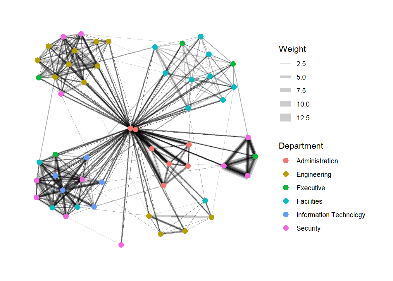
5 Plotting Practice - Creating facet graphs
5.1 Working with facet_edges()
Click to view the code.
set_graph_style()

g <- ggraph(GAStech_graph,
            layout = "nicely") +
  geom_edge_link(aes(width=Weight),
                 alpha=0.2) +
  scale_edge_width(range = c(0.1, 5)) +
  geom_node_point(aes(colour = Department),
                  size = 2)

g + facet_edges(~Weekday)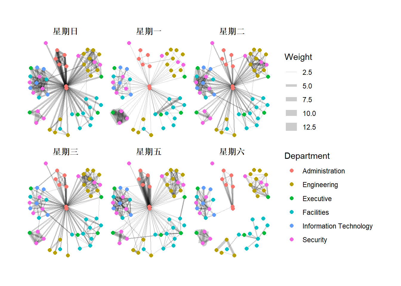
5.2 Working with facet_edges()
Click to view the code.
set_graph_style()

g <- ggraph(GAStech_graph,
            layout = "nicely") +
  geom_edge_link(aes(width=Weight),
                 alpha=0.2) +
  scale_edge_width(range = c(0.1, 5)) +
  geom_node_point(aes(colour = Department),
                  size = 2) +
  theme(legend.position = 'bottom')

g + facet_edges(~Weekday)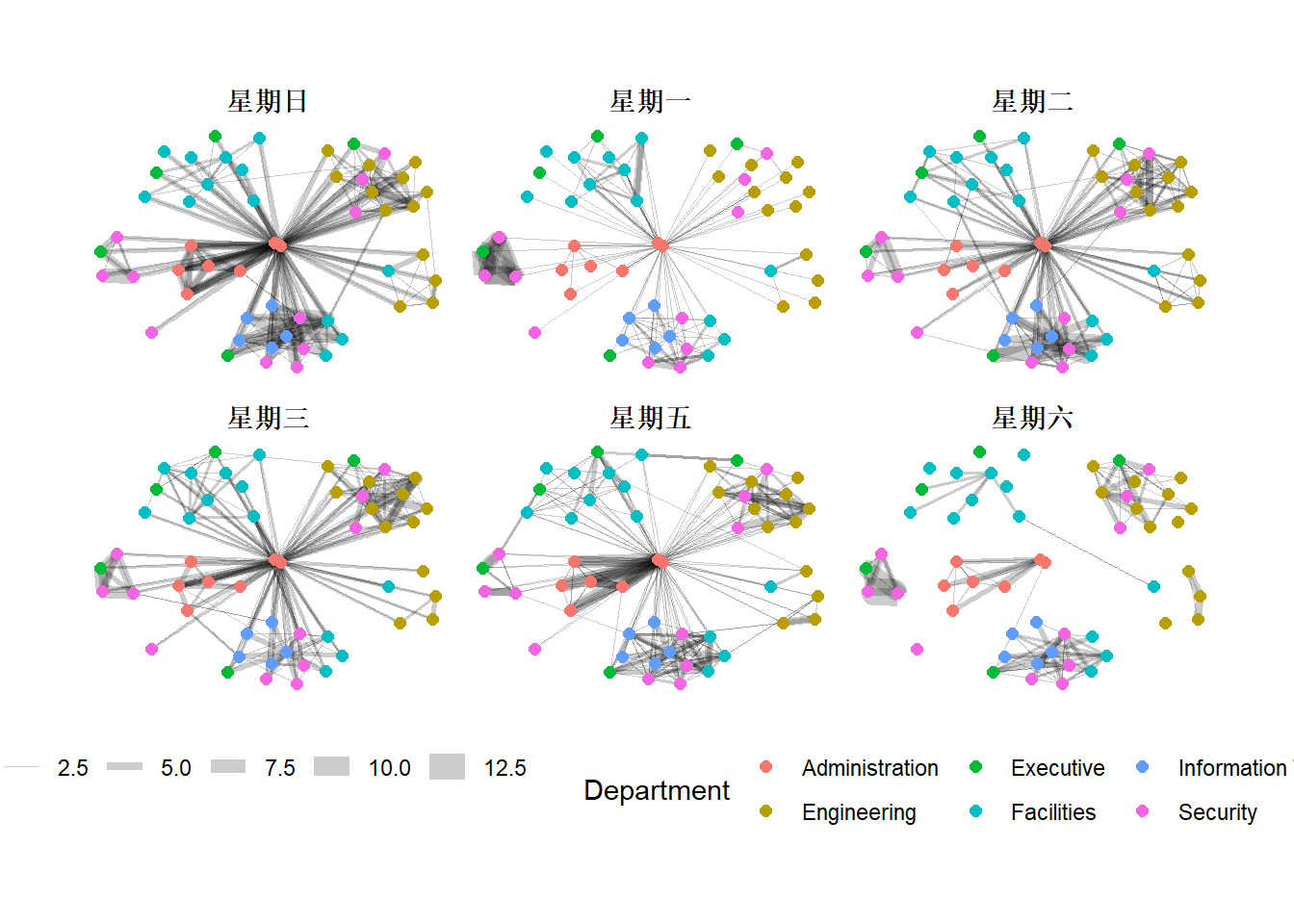
5.3 A framed facet graph
Click to view the code.
set_graph_style()

g <- ggraph(GAStech_graph,
            layout = "nicely") +
  geom_edge_link(aes(width=Weight),
                 alpha=0.2) +
  scale_edge_width(range = c(0.1, 5)) +
  geom_node_point(aes(colour = Department),
                  size = 2)

g + facet_edges(~Weekday) +
  th_foreground(foreground = "grey80",
                border = TRUE) +
  theme(legend.position = 'bottom')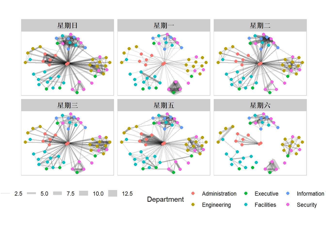
5.4 Working with facet_nodes()
Click to view the code.
set_graph_style()

g <- ggraph(GAStech_graph,
            layout = "nicely") +
  geom_edge_link(aes(width=Weight),
                 alpha=0.2) +
  scale_edge_width(range = c(0.1, 5)) +
  geom_node_point(aes(colour = Department),
                  size = 2)

g + facet_nodes(~Department)+
  th_foreground(foreground = "grey80",
                border = TRUE) +
  theme(legend.position = 'bottom')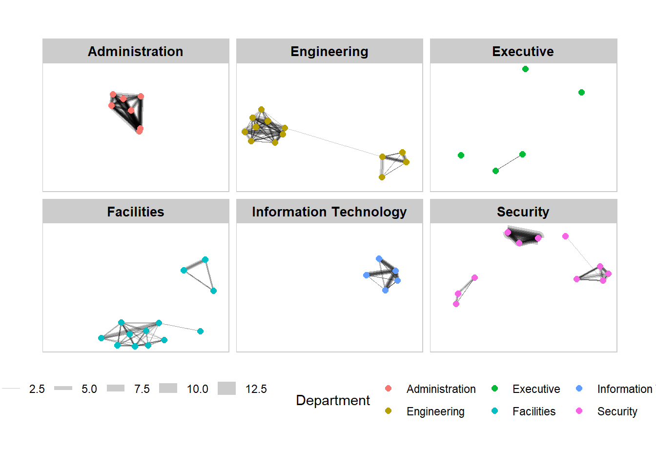
6 Plotting Practice - Network Metrics Analysis
6.1 Computing centrality indices
Click to view the code.
g <- GAStech_graph %>%
  mutate(betweenness_centrality = centrality_betweenness()) %>%
  ggraph(layout = "fr") +
  geom_edge_link(aes(width=Weight),
                 alpha=0.2) +
  scale_edge_width(range = c(0.1, 5)) +
  geom_node_point(aes(colour = Department,
            size=betweenness_centrality))
g + theme_graph()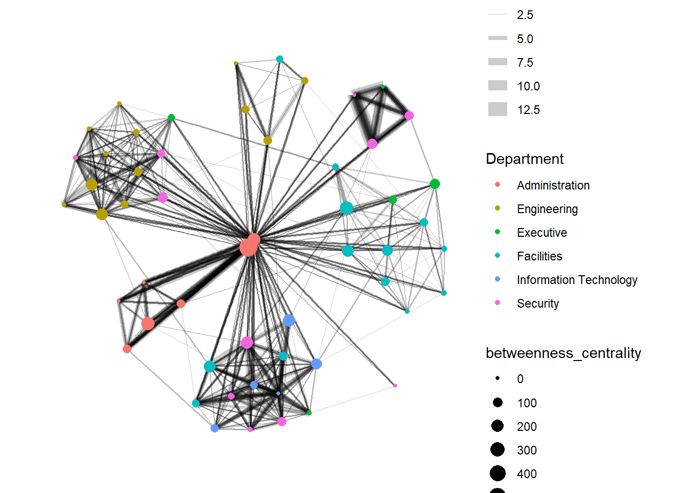
6.2 Visualising network metrics
Click to view the code.
g <- GAStech_graph %>%
  ggraph(layout = "fr") +
  geom_edge_link(aes(width=Weight),
                 alpha=0.2) +
  scale_edge_width(range = c(0.1, 5)) +
  geom_node_point(aes(colour = Department,
                      size = centrality_betweenness()))
g + theme_graph()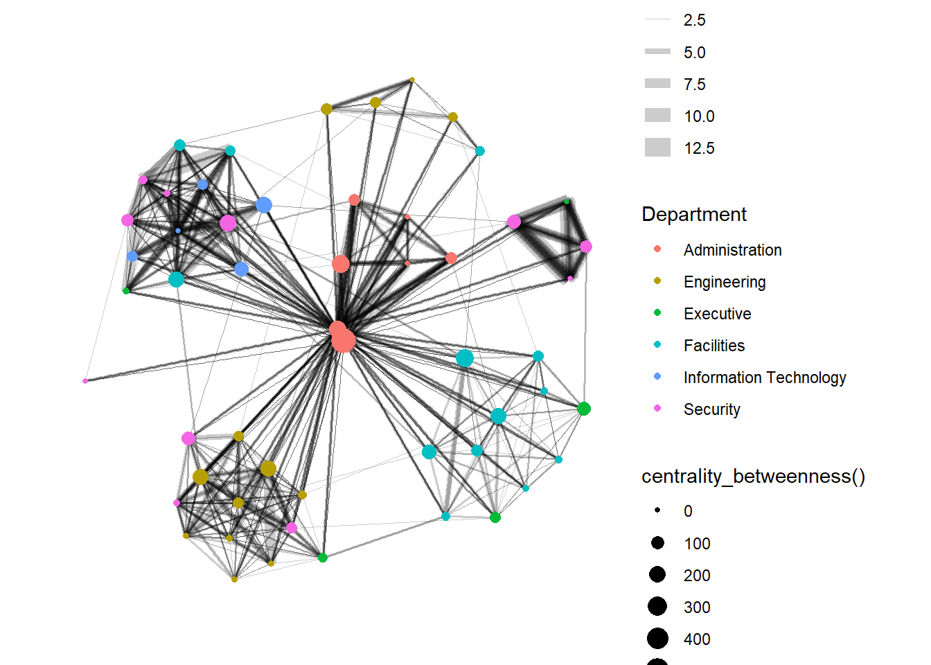
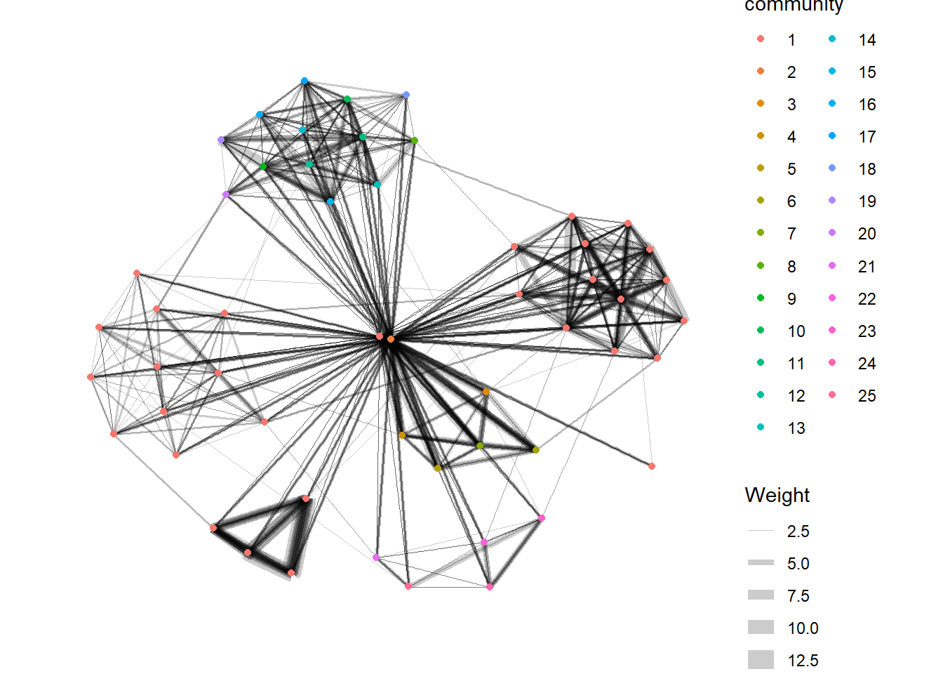
6.3 Visualising Community
Click to view the code.
7 Plotting Practice - Building Interactive Network Graph with visNetwork
7.1 Data preparation
Click to view the code.
GAStech_edges_aggregated <- GAStech_edges %>%
  left_join(GAStech_nodes, by = c("sourceLabel" = "label")) %>%
  rename(from = id) %>%
  left_join(GAStech_nodes, by = c("targetLabel" = "label")) %>%
  rename(to = id) %>%
  filter(MainSubject == "Work related") %>%
  group_by(from, to) %>%
    summarise(weight = n()) %>%
  filter(from!=to) %>%
  filter(weight > 1) %>%
  ungroup()
7.2 Plotting the first interactive network graph
Click to view the code.
visNetwork(GAStech_nodes,
           GAStech_edges_aggregated)
7.3 Working with layout
Click to view the code.
visNetwork(GAStech_nodes,
           GAStech_edges_aggregated) %>%
  visIgraphLayout(layout = "layout_with_fr")
7.4 Working with visual attributes - Nodes
Click to view the code.
GAStech_nodes <- GAStech_nodes %>%
  rename(group = Department)

visNetwork(GAStech_nodes,
           GAStech_edges_aggregated) %>%
  visIgraphLayout(layout = "layout_with_fr") %>%
  visLegend() %>%
  visLayout(randomSeed = 123)
7.5 Working with visual attributes - Edges
Click to view the code.
visNetwork(GAStech_nodes,
           GAStech_edges_aggregated) %>%
  visIgraphLayout(layout = "layout_with_fr") %>%
  visEdges(arrows = "to",
           smooth = list(enabled = TRUE,
                         type = "curvedCW")) %>%
  visLegend() %>%
  visLayout(randomSeed = 123)
7.6 Interactivity
Click to view the code.
visNetwork(GAStech_nodes,
           GAStech_edges_aggregated) %>%
  visIgraphLayout(layout = "layout_with_fr") %>%
  visOptions(highlightNearest = TRUE,
             nodesIdSelection = TRUE) %>%
  visLegend() %>%
  visLayout(randomSeed = 123)