Hands-on Exercise 4.2: Visual Statistical Analysis

1 Visual Statistical Analysis with ggstatsplot

ggstatsplot is an extension of ggplot2 package for creating graphics with details from statistical tests included in the information-rich plots themselves.

• To provide alternative statistical inference methods by default.

• To follow best practices for statistical reporting. For all statistical tests reported in the plots, the default template abides by the APA gold standard for statistical reporting. For example, here are results from a robust t-test:

1.1 Install and loading R packages.

pacman::p_load(ggstatsplot, tidyverse)

1.2 Importing the data

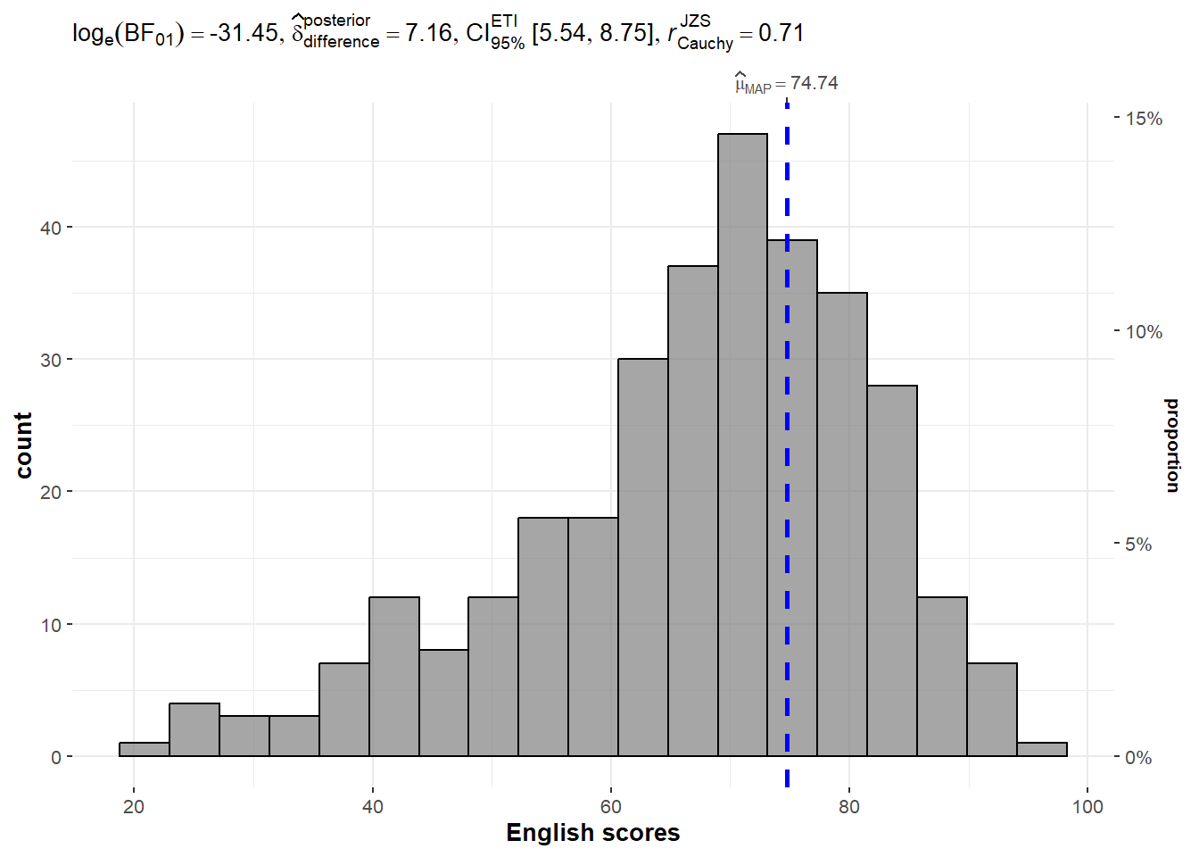
exam <- read_csv("../../data/Exam_data.csv")

1.3 One-sample test: gghistostats() method

In the code chunk below, gghistostats() is used to to build an visual of one-sample test on English scores.

Default information: - statistical details - Bayes Factor - sample sizes - distribution summary

set.seed(1234)

gghistostats(
  data = exam,
  x = ENGLISH,
  type = "bayes",
  test.value = 60,
  xlab = "English scores"
)

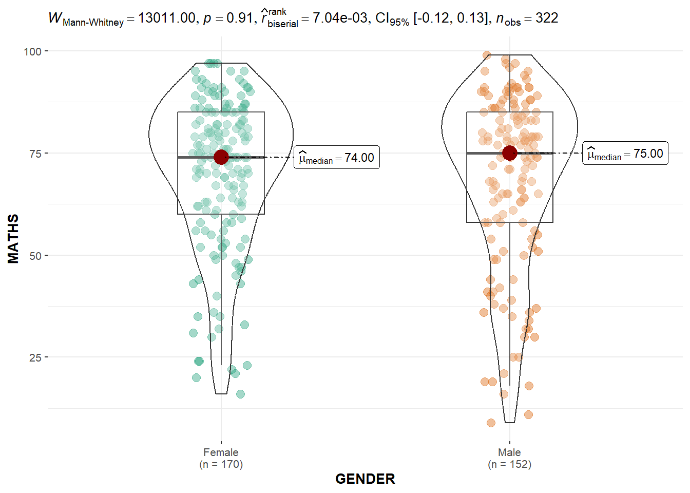
1.4 Two-sample mean test: ggbetweenstats()

In the code chunk below, ggbetweenstats() is used to build a visual for two-sample mean test of Maths scores by gender.

Default information: - statistical details - Bayes Factor - sample sizes - distribution summary

ggbetweenstats(
  data = exam,
  x = GENDER, 
  y = MATHS,
  type = "np",
  messages = FALSE
)

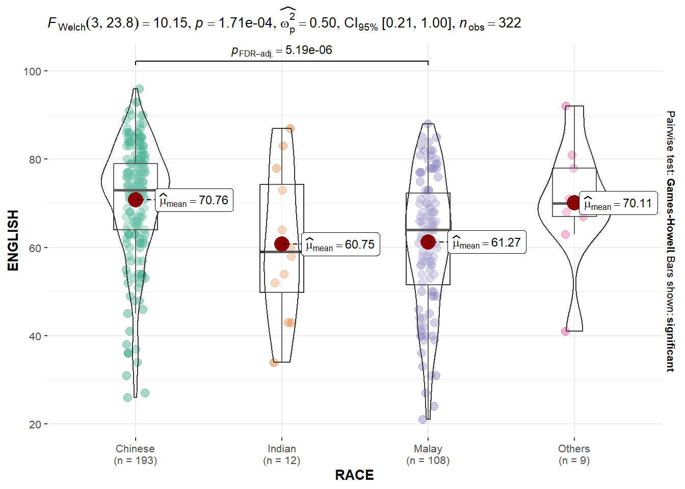
1.5 Oneway ANOVA Test: ggbetweenstats() method

In the code chunk below, ggbetweenstats() is used to build a visual for One-way ANOVA test on English score by race.

• “ns” → only non-significant

• “s” → only significant

• “all” → everything

ggbetweenstats(
  data = exam,
  x = RACE, 
  y = ENGLISH,
  type = "p",
  mean.ci = TRUE, 
  pairwise.comparisons = TRUE, 
  pairwise.display = "s",
  p.adjust.method = "fdr",
  messages = FALSE
)

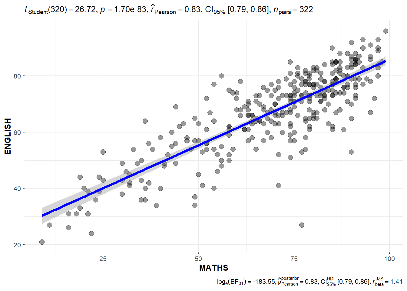
1.6 Significant Test of Correlation: ggscatterstats()

In the code chunk below, ggscatterstats() is used to build a visual for Significant Test of Correlation between Maths scores and English scores.

ggscatterstats(
  data = exam,
  x = MATHS,
  y = ENGLISH,
  marginal = FALSE,
  )

1.7 Significant Test of Association (Depedence) : ggbarstats() methods

In the code chunk below, the Maths scores is binned into a 4-class variable by using cut().

exam1 <- exam %>% 
  mutate(MATHS_bins = 
           cut(MATHS, 
               breaks = c(0,60,75,85,100))
)

In this code chunk below ggbarstats() is used to build a visual for Significant Test of Association

ggbarstats(exam1, 
           x = MATHS_bins, 
           y = GENDER)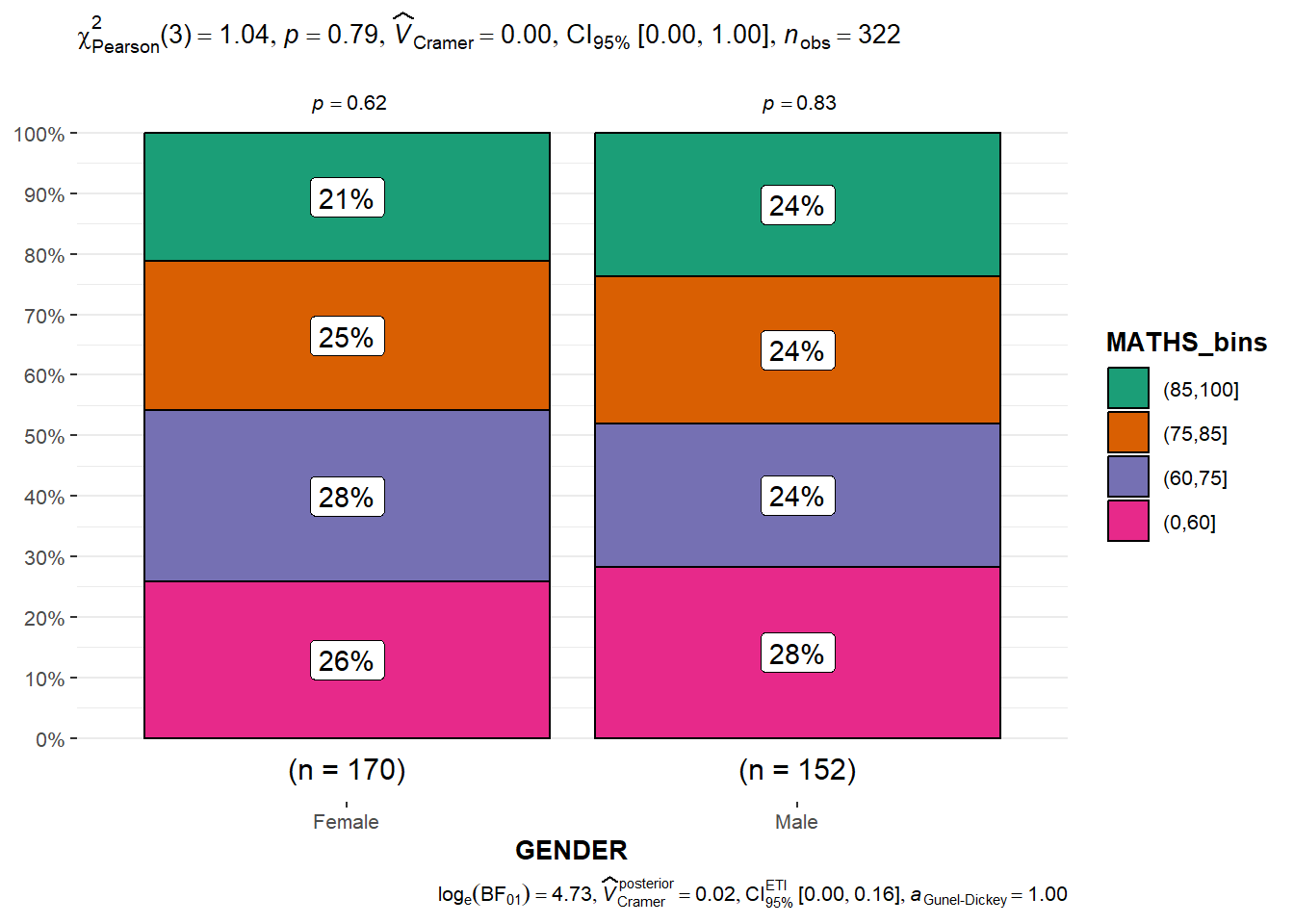

2 Visualising Models

Learning how to visualise model diagnostic and model parameters by using parameters package.

• Toyota Corolla case study will be used. The purpose of study is to build a model to discover factors affecting prices of used-cars by taking into consideration a set of explanatory variables.

2.1 Installing and loading the required libraries

pacman::p_load(readxl, performance, parameters, see)

2.2 Importing Excel file: readxl methods

In the code chunk below, read_xls() of readxl package is used to import the data worksheet of ToyotaCorolla.xls workbook into R.

car_resale <- read_xls("../../data/ToyotaCorolla.xls", 
                       "data")

2.3 Multiple Regression Model using lm()

The code chunk below is used to calibrate a multiple linear regression model by using lm() of Base Stats of R.

model <- lm(Price ~ Age_08_04 + Mfg_Year + KM + 
              Weight + Guarantee_Period, data = car_resale)
model

Call:
lm(formula = Price ~ Age_08_04 + Mfg_Year + KM + Weight + Guarantee_Period, 
    data = car_resale)

Coefficients:
     (Intercept)         Age_08_04          Mfg_Year                KM  
      -2.637e+06        -1.409e+01         1.315e+03        -2.323e-02  
          Weight  Guarantee_Period  
       1.903e+01         2.770e+01  

2.4 Model Diagnostic: checking for multicolinearity

In the code chunk, check_collinearity() of performance package.

check_collinearity(model)

check_c <- check_collinearity(model)
plot(check_c)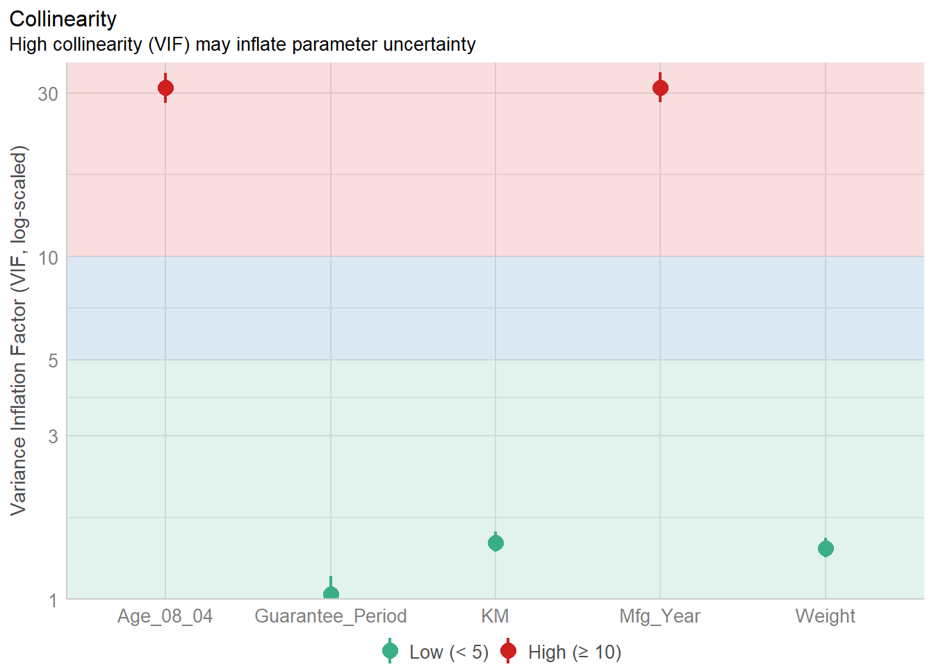

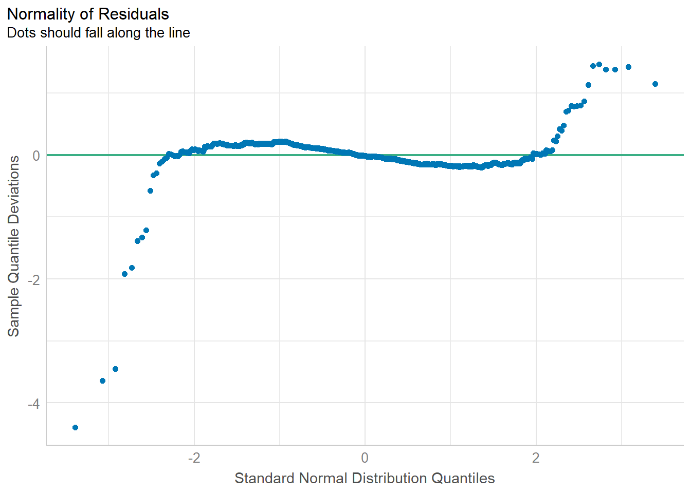
2.5 Model Diagnostic: checking normality assumption

In the code chunk, check_normality() of performance package.

model1 <- lm(Price ~ Age_08_04 + KM + 
              Weight + Guarantee_Period, data = car_resale)

check_n <- check_normality(model1)

plot(check_n)

2.6 Model Diagnostic: Check model for homogeneity of variances

In the code chunk, check_heteroscedasticity() of performance package.

check_h <- check_heteroscedasticity(model1)
plot(check_h)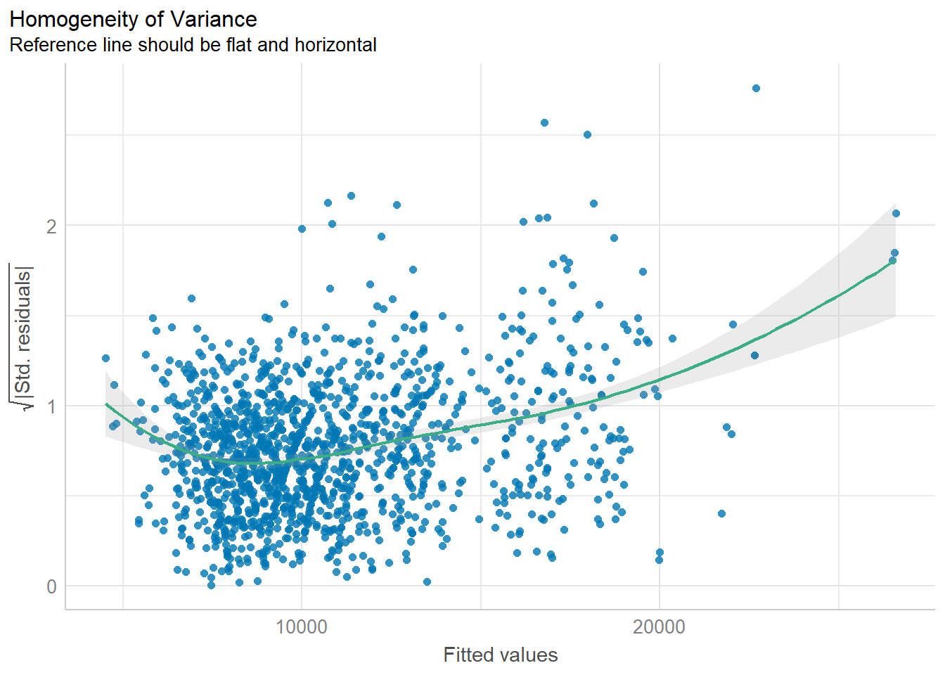

2.7 Model Diagnostic: Complete check

We can also perform the complete by using check_model().

check_model(model1)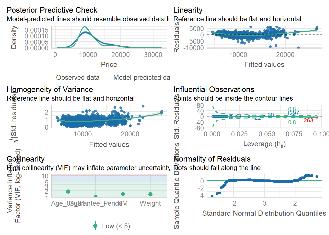

2.8 Visualising Regression Parameters: see methods

In the code below, plot() of see package and parameters() of parameters package is used to visualise the parameters of a regression model.

plot(parameters(model1))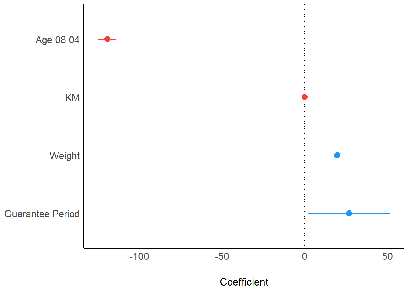

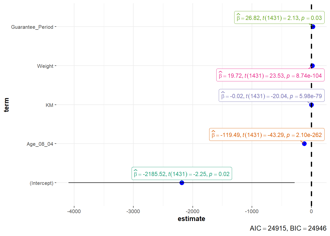
2.9 Visualising Regression Parameters: ggcoefstats() methods

In the code below, ggcoefstats() of ggstatsplot package to visualise the parameters of a regression model.

ggcoefstats(model1, 
            output = "plot")