In-class Exercise 7: Visualising and Analysing Geographic Data

View the slides to learn more about:

• Introducing map

• Properties of geographical data

• Typology of map

• Thematic mapping techniques

  • Proportional symbol map

  • Choropleth map

  • Data Classification

• Alternative mapping techniques

1 IsoMap

1.1 Loading R Package

pacman::p_load(sf, terra, gstat, tmap, viridis, tidyverse)

1.2 Dataset

rfstations <- read.csv("data/aspatial/RainfallStation.csv")

rfdata <- read_csv("data/aspatial/DAILYDATA_202402.csv") %>%
  select(c(1, 5)) %>%
  group_by(Station) %>%
  summarise(MONTHSUM = sum(`Daily Rainfall Total (mm)`)) %>%
  ungroup()

rfdata <- rfdata %>%
  left_join(rfstations)

rfdata_sf <- st_as_sf(rfdata,
                      coords = c("Longitude", "Latitude"),
                      crs = 4326) %>%
  st_transform(crs = 3414)

mpsz2019 <- st_read(dsn = "data/geospatial", layer = "MPSZ-2019") %>%
  st_transform(crs = 3414)

Reading layer `MPSZ-2019' from data source 
  `E:\kaixx1027\ISSS608-VAA\In-class_Ex\In-class_Ex07\data\geospatial' 
  using driver `ESRI Shapefile'
Simple feature collection with 332 features and 6 fields
Geometry type: MULTIPOLYGON
Dimension:     XY
Bounding box:  xmin: 103.6057 ymin: 1.158699 xmax: 104.0885 ymax: 1.470775
Geodetic CRS:  WGS 84

1.3 Visualisation

tmap_options(check.and.fix = TRUE)
tmap_mode("view")
tm_shape(mpsz2019)+
  tm_borders()+
  tm_shape(rfdata_sf)+
  tm_dots(col= 'MONTHSUM')

tmap_mode("plot")

grid <- terra::rast(mpsz2019,
                    nrows = 690,
                    ncols = 1075)

xy <-terra::xyFromCell(grid,
                       1:ncell(grid))

coop <-st_as_sf(as.data.frame(xy),
                coords = c("x","y"),
                crs = st_crs(mpsz2019))
coop <-st_filter(coop,mpsz2019)

res <- gstat(formula = MONTHSUM ~ 1,
             locations = rfdata_sf,
             nmax = 15,
             set = list(idp = 0))

resp<- predict(res,coop)

[inverse distance weighted interpolation]

resp$x<-st_coordinates(resp)[,1]
resp$y<-st_coordinates(resp)[,2]
resp$pred <-resp$var1.pred

pred<- terra::rasterize(resp,grid,
                        field="pred",
                        fun="mean")

tmap_options(check.and.fix = TRUE)
tmap_mode("plot")
tm_shape(pred)+
  tm_raster(alpha = 0.6,
            palette = "viridis")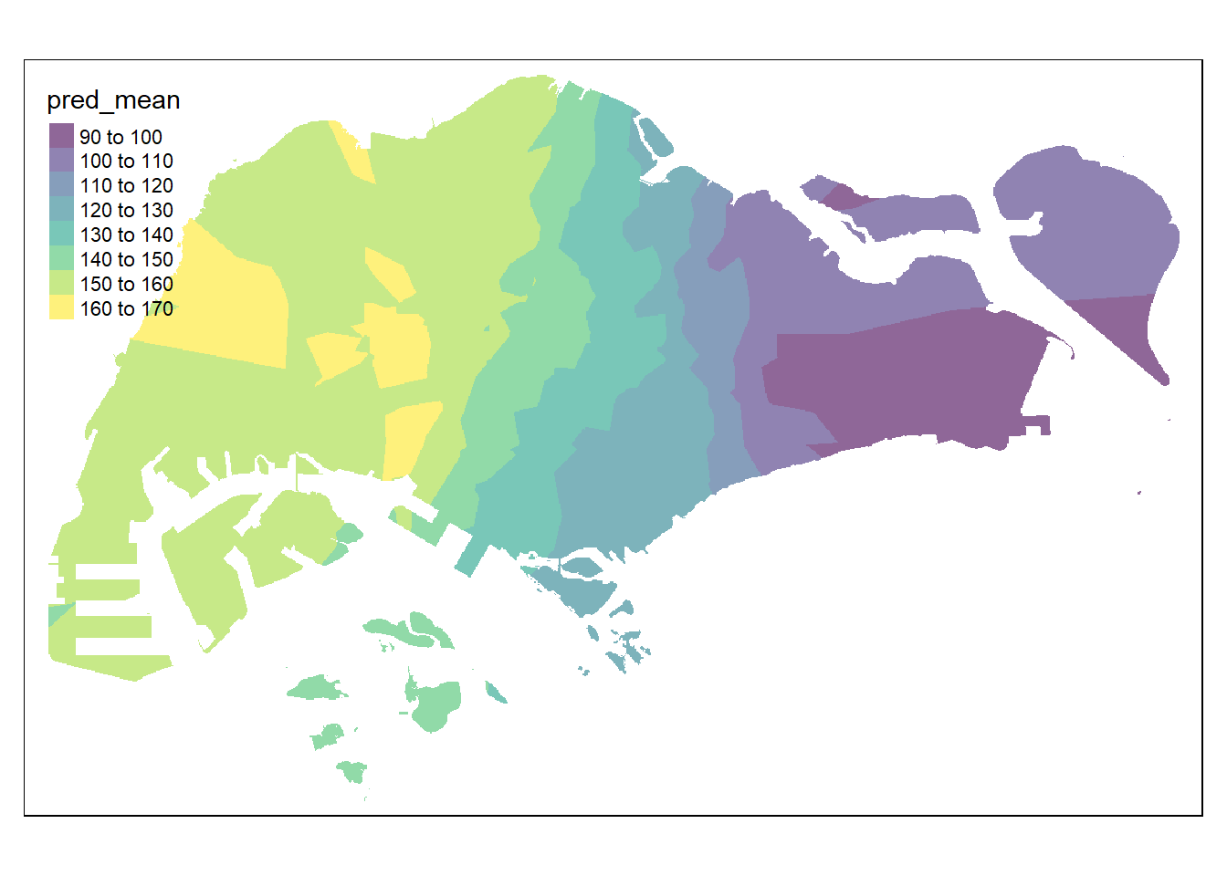

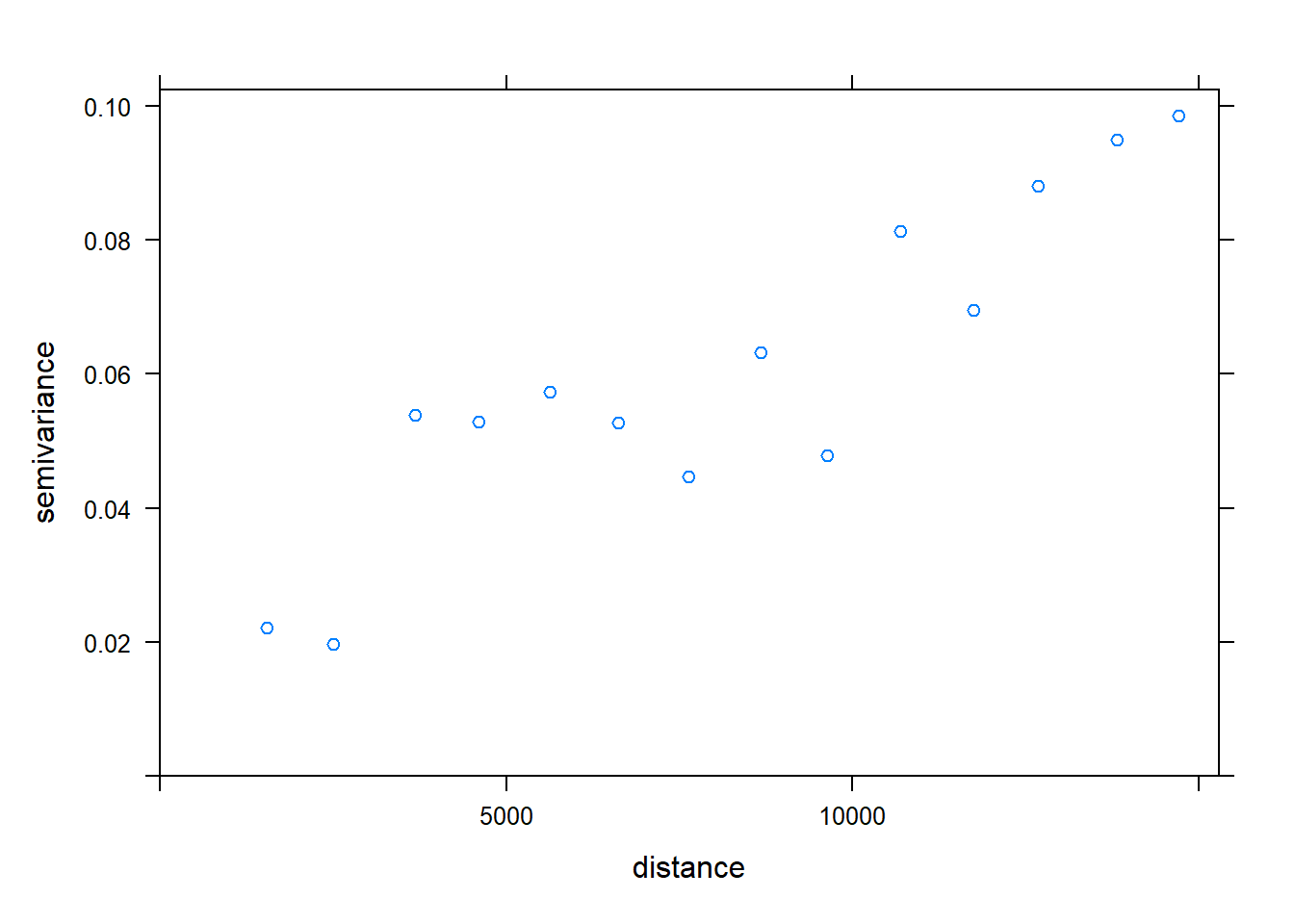
v<- variogram(log(MONTHSUM)~1,
              data = rfdata_sf)
plot(v)

fv<-fit.variogram(object = v,
                  model = vgm(psill = 0.5,model = "Sph",
                              range = 900,nugget = 0.1))
fv

plot(v,fv,cex =1.5)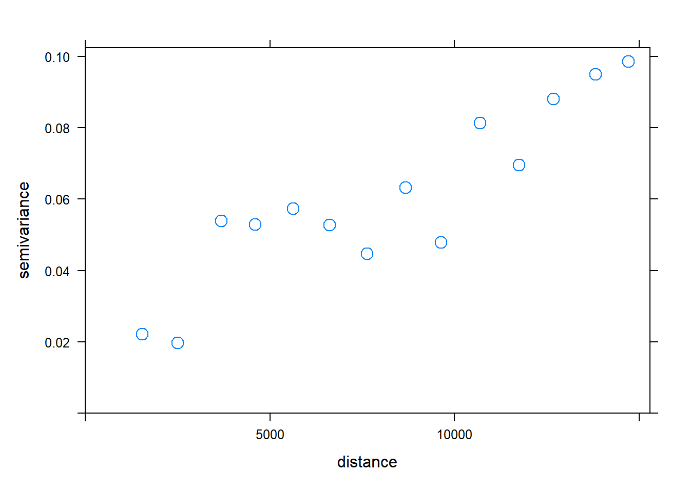

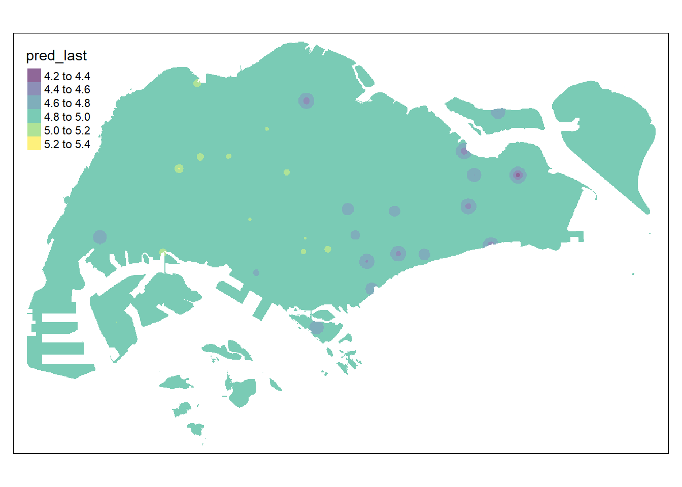
k<-gstat(formula = log(MONTHSUM)~1,
              data = rfdata_sf,
         model=fv)

resp<- predict(k,coop)

[using ordinary kriging]

resp$x<-st_coordinates(resp)[,1]
resp$y<-st_coordinates(resp)[,2]
resp$pred <-resp$var1.pred

kpred<- terra::rasterize(resp,grid,
                        field="pred")

tmap_options(check.and.fix = TRUE)
tmap_mode("plot")
tm_shape(kpred)+
  tm_raster(alpha = 0.6,
            palette = "viridis")